Multi-Objective Optimization with apsimNGpy

This tutorial demonstrates how to perform multi-objective optimization on an APSIM Next Generation model using the apsimNGpy.optimizer.moo module. You will learn two ways to specify decision variables and how to run an evolutionary optimization algorithm using pymoo. This approach enables you to explore trade-offs between objectives like crop yield and environmental outcomes.

Prerequisites

Make sure you have the following installed and configured:

APSIM Next Generation installed
Python 3.10+
apsimNGpy package (latest version)
Python packages: pymoo, matplotlib, numpy, and pandas

Step 1: Import required modules

from apsimNGpy.optimizer.moo import MultiObjectiveProblem, compute_hyper_volume, NSGA2
from pymoo.optimize import minimize
import matplotlib.pyplot as plt
from apsimNGpy.core.apsim import ApsimModel as Runner

Interpretation

Runner`: handles model simulation and editing. It is an apsimNGpy class
MultiObjectiveProblem: wraps your problem into a multi-objective one
NSGA2: a multi-objective genetic algorithm
minimize: will be used to minimize the objectives in the finals steps

Step 2: Initialize the APSIM model runner

You create a runner tied to a specific .apsimx model file. This runner manages simulation and parameter editing. Here, I a using the default maize template. Because it does not have nitrate leaching in its Report table, I have also added it.

runner = Runner("Maize")
runner.add_report_variable('[Soil].Nutrient.NO3.kgha[1] as nitrate', report_name='Report')

Step 3: Define Objective Functions

Objective functions take APSIM output (as a DataFrame) and return scalar values. You can define any number of such functions depending on the goals. If you have 3 objectives, then we expect 3 functions.

Important

Maximization objectives must be converted into minimization form by negating them (e.g., -f(x)), since the underlying optimization algorithms are designed to minimize objective functions.

def maximize_yield(df):
    return -df['Yield'].mean()

def minimize_nitrate_leaching(df):
    return df['nitrate'].sum()

Step 4a: Define decision variables (Approach 1 - direct List)

You can directly supply a list of variables to optimize as follows:.

decision_vars = [
    {'path': '.Simulations.Simulation.Field.Fertilise at sowing',
     'Amount': "?", 'bounds': [50, 300], 'v_type': 'float'},

    {'path': '.Simulations.Simulation.Field.Sow using a variable rule',
     'Population': "?", 'bounds': [4, 14], 'v_type': 'float'}
]
# initialise the problem
problem = MultiObjectiveProblem(runner, objectives=[maximize_yield, minimize_nitrate_leaching], decision_vars=decision_vars)

Each dictionary defines:

path: the APSIM model path to the component.
Amount / Population: the parameter to be optimized (denoted by ‘?’).
bounds: lower and upper bounds for the optimizer.
v_type: variable type.

Note

Each decision variable specification must contain exactly one parameter marked with '?'. This signifies the target parameter to be optimized during the calibration or search process.

Step 3b: Define decision variables (Approach 2 - using `.add_parameters()`)

Instead of a list, you can add each parameter one at a time. There is a need to initiate our problem with objectives only, then add control variables on the fly.

# initialise the problem
problem = MultiObjectiveProblem(runner, objectives=[maximize_yield, minimize_nitrate_leaching])

problem.add_parameters(
    path='.Simulations.Simulation.Field.Fertilise at sowing',
    Amount='?', bounds=[50, 300], v_type='float')

problem.add_parameters(
    path='.Simulations.Simulation.Field.Sow using a variable rule',
    Population='?', bounds=[4, 14], v_type='float')

Note

The best approach depends on the user’s preference, but the last approach helps the user to focus on one control variables required details at a time.

Step 5: Run the NSGA-II optimizer

NSGA-II is a commonly used algorithm for multi-objective problems. There are other genetic multi-objective algorithms, but for trade-off analysis with APSIM, NSGA-II is more than adequate. You can now run it as follows:

algorithm = NSGA2(pop_size=20)

result = minimize(
    problem.get_problem(),
    algorithm,
    ('n_gen', 10),
    seed=1,
    verbose=True
)

pop_size: number of candidate solutions per generation.
n_gen: number of generations to run.

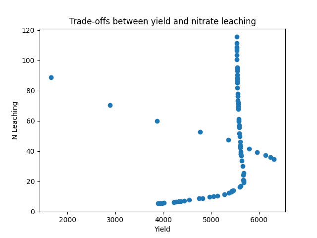
Step 6: Plot the Pareto Front

The results show trade-offs between competing objectives. You can visualize them:

F = result.F
plt.scatter(F[:, 0]* -1, F[:, 1])
plt.xlabel("Yield")
plt.ylabel("N Leaching")
plt.title("Pareto Front")
plt.show()

comment

From the graph above, it is clear that achieving high corn yield while simultaneously reducing nitrate leaching is quite challenging. This is because high yields typically require the application of large amounts of nitrogen fertilizer, which is often associated with increased nitrate leaching.

Tip

Compute Hyper volume (Optional)

The hyper volume gives a scalar metric of solution quality, and can be useful if you want to explore the best inputs such as pop_size, max_gen.

A high value indicates better solution quality than a lower one. Therefore, it can also be used to compare the performance of multiple minimization algorithms.

hv = compute_hyper_volume(F, normalize=True)
print("Hyper volume:", hv)

Hint

Objectives are typically expressed in different units, and some—such as yield—may have much larger amplitudes. This makes determining a suitable reference point challenging. In such cases, normalization can help automatically detect the reference point by applying specific thresholds.

Comparing objectives without mult-objective optimization

What if we just run out the different combinations of the decision variables: population density and the nitrogen application rate can we ge the same pareto front and trade-offs we have seen in that graph? To answer this question we are going to run a factorial experiment.

import numpy as np
population  = [str(i) for i in np.random.randint(low=1, high=12, size=20)]
nitrogen  = [str(i) for i in np.random.randint(low=50, high=300, size=20)]
runner.create_experiment(permutation=False, base_name='Simulation')
runner.add_factor(specification=f"[Fertilise at sowing].Script.Amount = {','.join(nitrogen)}", factor_name='Nitrogen')
runner.add_factor(specification=f"[Sow using a variable rule].Script.Population ={','.join(population)}",
                 factor_name='Population')
runner.run(verbose=True)

df = runner.results.drop_duplicates()
df  = df.groupby('SimulationID')[['Yield', 'nitrate']].mean()
yi = df.Yield
nitrate  =df.nitrate
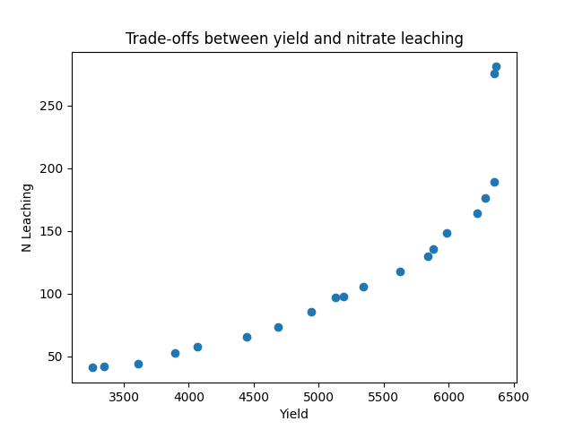
plt.scatter(yi , nitrate)
plt.xlabel("Yield")
plt.ylabel("N Leaching")
plt.title("Trade-offs between yield and nitrate leaching")
plt.show()