Automatic Parameter calibration
This tutorial demonstrates how to automatically calibrate APSIM parameters using the optimization algorithms
available in apsimNGpy. For detailed information on defining and submitting optimization factors,
refer to the API documentation for submit_factor().
from apsimNGpy.core.config import apsim_bin_context
# The modules below may require proper APSIM binary path specification install
from apsimNGpy.optimizer.minimize.single_mixed import MixedVariableOptimizer
from apsimNGpy.optimizer.problems.smp import MixedProblem
from apsimNGpy.tests.unittests.test_factory import obs# mimics observed data
from apsimNGpy.optimizer.problems.variables import UniformVar, QrandintVar
Some algorithms like Differential Evolution can be set to run in parallel, therefore everything needs to be executed below the module guard
Defining the Optimization Problem
To define an optimization problem that identifies the optimum APSIM parameters, use the class MixedProblem.
This class accepts an APSIM template file, a training (observed) dataset, and the corresponding index variables linking observed and simulated data.
A key requirement is to specify a performance metric that serves as the optimization target. This metric guides the algorithm in assessing model performance and convergence quality. Commonly used metrics include WIA, RMSE, RRMSE, Bias, CCC, R², Slope, ME, and MAE.
An example usage is shown below.
if __name__ == "__main__":
    # -------------------------------------------------------------
    # 1. Define the mixed-variable optimization problem
    # -------------------------------------------------------------
    mp = MixedProblem(
        model="Maize",
        trainer_dataset=obs,
        pred_col="Yield",
        metric="wia",
        index="year",
        table = 'Report',
        trainer_col="observed"
    )
Defining the factors
Once the optimization problem is instantiated, the remaining task is to submit the factors, the parameters that will be sampled during the search process. These factors finalize the problem specification and determine the parameter space over which the optimization algorithm will operate.
Each factor requires a set of python parameters that define how it will be sampled and handled by apsimNGpy execution engine. For example, the dictionary below specifies the target model path, the variable type and sampling range, the starting value, the candidate parameter to modify, and any additional parameters needed by the APSIM model component.
soil_param = {
    "path": ".Simulations.Simulation.Field.Soil.Organic",
    "vtype": [UniformVar(1, 200)],
    "start_value": [1],
    "candidate_param": ["FOM"],
    "other_params": {"FBiom": 0.04, "Carbon": 1.89},
}
In general as seen in the example above, the keys in the dictionary above can be broken down as follows;
path: a fully qualified model path pointing to the APSIM component to be edited. For extracting this path, please see inspect model section
vtype: A list defining the variable types used for sampling parameter values (e.g.,
UniformVar,GridVar,CategoricalVar). Variable types may also be provided as strings.ChoiceVar(items) Nominal (unordered categorical) Example:
ChoiceVar(["A", "B", "C"])GridVar(values) Ordinal (ordered categorical) Example:
GridVar([2, 4, 8, 16])RandintVar(lower, upper) Integer in
[lower, upper]Example:RandintVar(0, 6)QrandintVar(lower, upper, q) Quantized integer with step
qExample:QrandintVar(0, 12, 3)UniformVar(lower, upper) Continuous float range Example:
UniformVar(0.0, 5.11)QuniformVar(lower, upper, q) Quantized float with step
qExample:QuniformVar(0.0, 5.1, 0.3)
Below is a list of allowable string names for each variable type. For further details, see
submit_factor().ALLOWED_VARIABLES = { # Original canonical names "UniformVar": UniformVar, "QrandintVar": QrandintVar, "QuniformVar": QuniformVar, "GridVar": GridVar, "ChoiceVar": ChoiceVar, "RandintVar": RandintVar, # Short aliases "uniform": UniformVar, "quniform": QuniformVar, "qrandint": QrandintVar, "grid": GridVar, "choice": ChoiceVar, "randint": RandintVar, # Descriptive aliases (readable English) "continuous": UniformVar, "quantized_continuous": QuniformVar, "quantized_int": QrandintVar, "ordinal": GridVar, "categorical": ChoiceVar, "integer": RandintVar, # Alternative descriptive (for domain users) "step_uniform_float": QuniformVar, "step_random_int": QrandintVar, "ordered_var": GridVar, "choice_var": ChoiceVar }
start_value: A list of initial parameter values. Each entry corresponds to one parameter within the factor definition and is used to seed the optimizer or establish a baseline.
- candidate_param: list or tuple of str Names of APSIM variables (e.g.,
"FOM","FBiom") to be optimized. These must exist within the APSIM node path.
- candidate_param: list or tuple of str Names of APSIM variables (e.g.,
other_params: dict — Additional APSIM constants to fix during optimization (non-optimized). These must belong to the same APSIM node. For example, when optimizing
FBiombut also modifyingCarbon, supplyCarbonunderother_paramsFor details seeedit_model_by_path()- cultivar: bool Indicates whether the parameter belongs to a cultivar node. Set to
Truewhen defining cultivar-related optimization factors.
Tip
Each distinct node on APSIM should appear in one single entry or submission, hence if they are multiple paramters on a single node, they should all be defined by a single entry
When a factor contains multiple parameters, the fields
vtype,start_value, andcandidate_paramprovided as a list must be the same size as the number of parameters to optimize on that node and should be the same length
For the example above, if multiple parameters at the same model path need to be optimized, they can be defined as follows:
soil_param = {
    "path": ".Simulations.Simulation.Field.Soil.Organic",
    "vtype": [UniformVar(1, 200), UniformVar(1, 3)],
    "start_value": [1, 2],
    "candidate_param": ["FOM", 'Carbon'],
    "other_params": {"FBiom": 0.04, },
}
Cultivar-specific parameters can be defined as shown below. Note that if you do not explicitly set cultivar=True, the factor may still pass Pydantic validation, but it will not be recognized correctly by apsimNGpy. As a result, an error will be raised when the optimizer starts.
cultivar_param = {
    "path": ".Simulations.Simulation.Field.Maize.CultivarFolder.Dekalb_XL82",
    "vtype": [ QrandintVar(400, 900, q=10), UniformVar(0.8,2.2)],  # Discrete step size of 10 for the first factor
    "start_value": [ 600, 1],
    "candidate_param": [
                        '[Phenology].GrainFilling.Target.FixedValue',
                        '[Leaf].Photosynthesis.RUE.FixedValue'],
    "other_params": {"sowed": True},
    "cultivar": True,  # Signals to apsimNGpy to treat it as a cultivar parameter
}
Cultivar specific paramters are still tricky, as there is need to specify whether the cultivar to be edited is the one specified in the manager script managing the sowing operations. There are also situations where you may want to optimize the parameters of a cultivar that is not the one currently specified in the manager script. In such cases, you have two options. The first option is to explicitly indicate that the cultivar is not yet sown in the simulation, while also providing the path to the manager script responsible for sowing it. This ensures that apsimNGpy updates the cultivar name dynamically during optimization.
An example configuration is shown below:
cultivar_param = {
    "path": ".Simulations.Simulation.Field.Maize.CultivarFolder.Dekalb_XL82",
    "vtype": [
        QrandintVar(400, 900, q=10),
        UniformVar(0.8, 2.2)
    ],
    "start_value": [600, 1],
    "candidate_param": [
        "[Phenology].GrainFilling.Target.FixedValue",
        "[Leaf].Photosynthesis.RUE.FixedValue"
    ],
    "other_params": {
        "sowed": False,
        "manager_path": ".Simulations.Simulation.Field.Sow using a variable rule",
        "manager_param": "CultivarName",
    },
    "cultivar": True,  # Informs apsimNGpy that this is a cultivar-based parameter set
}
A more recommended and straightforward approach is to update the
``CultivarName`` in the manager script to the cultivar you intend to
calibrate, and then proceed exactly as in the first example. This avoids
the need to specify sowed=False and providing extra information such as the manager script path, and the associated param name.
The following example demonstrates how to modify the cultivar name programmatically before defining the optimization problem, but you can also do this in the GUI
from apsimNGpy.core.apsim import ApsimModel

# Load your APSIM template (replace with your actual template path)
model = ApsimModel("Maize")

# Update the cultivar used in the sowing manager rule
model.edit_model_by_path(
    path=".Simulations.Simulation.Field.Sow using a variable rule",
    CultivarName="Dekalb_XL82"
)

# After editing, extract the updated model path for use in the optimization setup
edited_path = 'edited_path.apsimx'
model.save(edited_path, reload =False) # no need to reload it back in memory
Use edited_path in the problem definition above when specifying the
template for calibration. This ensures that when defining the associated factors, we just signal that cultivar is sowed and no extra arguments are needed.
Note
If you are using Operations, it is not currently supported
Submit optimization factors
mp.submit_factor(**soil_param)
# submit the cultivar one
mp.submit_factor(**cultivar_param)

print(f" {mp.n_factors} optimization factors registered.")
 #4 optimization factors registered.")
without value unpacking, we can submit variables directly as follows:
mp.mp.submit_factor(
    path=".Simulations.Simulation.Field.Maize.CultivarFolder.Dekalb_XL82",
    vtype=[
        QrandintVar(400, 900, q=10),
        UniformVar(0.8, 2.2),
    ],
    start_value=[600, 1],
    candidate_param=[
        "[Phenology].GrainFilling.Target.FixedValue",
        "[Leaf].Photosynthesis.RUE.FixedValue",
    ],
    other_params={
        "sowed": False,
        "manager_path": ".Simulations.Simulation.Field.Sow using a variable rule",
        "manager_param": "CultivarName",
    },
    cultivar=True,  # Informs apsimNGpy that this is a cultivar-based parameter set
)
There is still a chance to submit all defined factors at once
mp.submit_all([soil_param,cultivar_param ])
Submitting untyped factors
Factors may be submitted without explicitly specifying a variable type (e.g., UniformVar or ChoiceVar). In this case, all submitted factors are treated as continuous (float) variables by default. This approach is appropriate when the decision variables are purely numeric and bounded, and it avoids the additional overhead of defining explicit variable-type wrappers. An example of this usage is shown below:
mp.submit_factor(path='.Simulations.Replacements.Maize.OPVPH4edited',
                         candidate_param=[
                             '[Leaf].Photosynthesis.RUE.FixedValue',
                             '[Phenology].GrainFilling.Target.FixedValue',
                             '[Phenology].Juvenile.Target.FixedValue',
                             '[Phenology].FloweringToGrainFilling.Target.FixedValue'
                         ],
                         bounds=[[1, 2.4], [600, 850], [200, 260], [100,200]],
                         start_value=[ 1.8, 800,200, 100],
                         other_params={'sowed':True},
                         cultivar=True)
Note
The code examples above are intended only to demonstrate how factors can be submitted to the optimizer. In this tutorial, however, only cultivar parameters were actually passed to the optimizer for calibration. All other factors shown in the examples are for illustration purposes and were not included in the optimization example below.
Tip
All submitted factors are validated using Pydantic.
- to ensure adherence to expected data structures and variable types — for example checking that
vtypeincludes valid variable types (UniformVar,GridVar), ensuringpathis a valid string, and that start_values is a string.After Pydantic validation, an additional structural check ensures that the lengths of
vtype,start_value, andcandidate_paramare identical. Each candidate parameter must have a matching variable type and initial value.In cases where
other_paramshas identical names ascandidate_param, thecandidate_paramtakes priority and the identical parameter is decoupled from the other_paramsOptimization methods that do not require bounded or initialized start values allow for dummy entries in
start_value. These placeholders are accepted without affecting the optimization process. The system remains flexible across both stochastic and deterministic search methods.
Configure the optimizer
minim = MixedVariableOptimizer(problem=mp)
Use differential evolution
apsimNGpy provides a high-level wrapper for Differential Evolution
(DE), enabling robust APSIM calibration without requiring users to
manage low-level evolutionary mechanics. DE is well suited to the
irregular, nonlinear parameter landscapes common in crop and soil
model calibration. Its population-based search balances broad
exploration with fine-scale refinement. Effective performance is
typically achieved using moderate population sizes (20–40), but you may consider making the population as 10 * number of parameters, mutation
factors between 0.6 and 0.9, and crossover rates between 0.7 and
0.9. For metrics where larger values indicate improved model
performance (such as WIA, CCC, R², and slope), apsimNGpy internally
transforms the problem into a minimization task, which requires
negative constraint bounds. Parallel execution via the workers
argument is essential for reducing computation time during APSIM
simulations.
Note
The observed dataset (obs) was generated using the maize cultivar
Dekalb_XL82, with the following true parameter values:
[Phenology].GrainFilling.Target.FixedValue = 813 and
[Leaf].Photosynthesis.RUE.FixedValue = 2.0.
Therefore, an effective optimization algorithm should be able to
recover parameter values that closely match these targets when
calibrating against the observed data.
de = minim.minimize_with_de(
    use_threads=True,
    updating="deferred", # recommended if workers > 1, otherwise use 'immediate'
    workers=14,
    popsize=30,
    maxiter=15,  # ~generations
    tol=1e-6,
    mutation=(0.5, 1.0),  # differential weight (can be tuple for dithering)
    recombination=0.7,  # crossover prob
    seed=42,  # reproducibility
    polish=True,  # local search at the end (uses L-BFGS-B) or trust-constr if the problem ahs constraint
    constraints=(-1.1, -0.8))
print(de)
result retrieval
After optimization is completed, we can print the instance of the minimization and for the above code see example below,
please note the illustration did not include the soil params, because of time constraints.
    message: Optimization terminated successfully.
            success: True
                fun: -0.9999574183647046
                  x: (800, 1.9847370688789152)
                nit: 5
               nfev: 604
         population: [[ 7.788e+02  1.983e+00]
                      [ 8.787e+02  2.092e+00]
                      ...
                      [ 7.743e+02  1.998e+00]
                      [ 7.054e+02  1.980e+00]]
population_energies: [-1.000e+00 -9.978e-01 ... -9.998e-01 -9.995e-01]
             constr: [array([ 0.000e+00])]
   constr_violation: 0.0
              maxcv: 0.0
                jac: [array([[-3.952e-06,  1.323e-03]]), array([[ 1.000e+00,  0.000e+00],
                            [ 0.000e+00,  1.000e+00]])]
             x_vars: [Phenology].GrainFilling.Target.FixedValue: 800
                           [Leaf].Photosynthesis.RUE.FixedValue: 1.9847370688789152
        all_metrics:  RMSE: 35.8565186378257
                       MAE: 27.500786187035384
                       MSE: 1285.689928824742
                     RRMSE: 0.006361340117450984
                      bias: 0.791396068637448
                        ME: 0.9998296586187999
                       WIA: 0.9999574183647046
                        R2: 0.9998297877255155
                       CCC: 0.9999148445037384
                     SLOPE: 1.000044541525716
               data:    year  observed        Yield
                     0  1991  8469.616  8525.106322
                     1  1992  4674.820  4666.814543
                     2  1993   555.017   550.891724
                     3  1994  3504.282  3505.616103
                     4  1995  7820.120  7748.800048
                     5  1996  8823.516  8856.269351
                     6  1997  3802.295  3854.178136
                     7  1998  2943.070  2926.598323
                     8  1999  8379.928  8361.239740
                     9  2000  7393.633  7378.696671
Highlight
Under the default parameter settings, result from DE algorithms was acceptable but at a very higher cost of 604 function evaluations
Tip
Differential Evolution (DE) is computationally intensive, especially when the number of parameters (decision variables) is large. Each generation evaluates the full population of candidate solutions, which can significantly increase computation time for APSIM-based calibration. In many cases, simpler local optimization algorithms (e.g., Nelder–Mead, Powell, or L-BFGS-B) may achieve comparable performance with far fewer evaluations. Users are encouraged to try these lower-cost local methods first, and adopt DE only when local algorithms consistently fail to identify satisfactory solutions or when the objective landscape is highly irregular or multi-modal.
Local optimization examples
Below are the results from one of the several local optimization algorithms included
in apsimNGpy. These methods generally
require far fewer APSIM evaluations.
nelda = minim.minimize_with_local(method="Nelder-Mead")
print(nelda)
nelda-mead
        message: Optimization terminated successfully.
       success: True
        status: 0
           fun: -0.9999978063483224
             x: (810, 1.9956845806066088)
           nit: 74
          nfev: 157
 final_simplex: (array([[ 8.086e+02,  1.996e+00],
                       [ 8.086e+02,  1.996e+00],
                       [ 8.086e+02,  1.996e+00]]), array([-1.000e+00, -1.000e+00, -1.000e+00]))
        x_vars: [Phenology].GrainFilling.Target.FixedValue: 810
                      [Leaf].Photosynthesis.RUE.FixedValue: 1.9956845806066088
   all_metrics:  RMSE: 8.142916753128027
                  MAE: 6.182601974125896
                  MSE: 66.30709324837308
                RRMSE: 0.001444642842712912
                 bias: 0.2038095028286307
                   ME: 0.9999912149565816
                  WIA: 0.9999978063483224
                   R2: 0.9999926474869694
                  CCC: 0.9999956129811112
                SLOPE: 1.0011872254349912
          data:    year  observed        Yield
                0  1991  8469.616  8466.879175
                1  1992  4674.820  4668.921189
                2  1993   555.017   552.965145
                3  1994  3504.282  3500.529818
                4  1995  7820.120  7814.047377
                5  1996  8823.516  8839.941004
                6  1997  3802.295  3800.652670
                7  1998  2943.070  2942.571063
                8  1999  8379.928  8395.435053
                9  2000  7393.633  7386.392601
Highlight
The Nelder–Mead solution provides a near-perfect fit (WIA ≈ 0.999998) using only 157 evaluations, compared to 604 for DE. The resulting RMSE of approximately 8 kg ha⁻¹ is effectively negligible, and the estimated slope is essentially 1.0. Together, these indicators demonstrate that the Nelder–Mead algorithm solved this calibration problem with exceptional precision.
powell = minim.minimize_with_local(method="Powell")
print(powell)
    Powell      message: Optimization terminated successfully.
    success: True
     status: 0
        fun: -0.9999978063480863
          x: (810, 1.9956853031734851)
        nit: 3
      direc: [[ 1.778e-04  8.225e-06]
              [ 1.256e+02  5.083e-02]]
       nfev: 156
     x_vars: [Phenology].GrainFilling.Target.FixedValue: 810
                   [Leaf].Photosynthesis.RUE.FixedValue: 1.9956853031734851
all_metrics:  RMSE: 8.142918248897413
               MAE: 6.181338616665698
               MSE: 66.3071176082265
             RRMSE: 0.0014446431080788248
              bias: 0.20602073354134517
                ME: 0.9999912149533542
               WIA: 0.9999978063480863
                R2: 0.9999926482235774
               CCC: 0.9999956129866351
             SLOPE: 1.0011874855510992
       data:    year  observed        Yield
             0  1991  8469.616  8466.882313
             1  1992  4674.820  4668.923545
             2  1993   555.017   552.965793
             3  1994  3504.282  3500.531051
             4  1995  7820.120  7814.050446
             5  1996  8823.516  8839.943474
             6  1997  3802.295  3800.654636
             7  1998  2943.070  2942.572631
             8  1999  8379.928  8395.437323
             9  2000  7393.633  7386.395996
Highlight
Powell achieved the same objective value as Nelder–Mead and also used about four times fewer evaluations than DE.
lbfgs = minim.minimize_with_local(method="L-BFGS-B", options={
    "gtol": 1e-12,
    "ftol": 1e-12,
    "maxfun": 50000,
    "maxiter": 30000
})

print(lbfgs)
     L-BFGS-B
     message: CONVERGENCE: RELATIVE REDUCTION OF F <= FACTR*EPSMCH
    success: True
     status: 0
        fun: -0.9988328727487307
          x: (600, 1.9146364126155142)
        nit: 5
        jac: [ 0.000e+00  1.443e-06]
       nfev: 51
       njev: 17
   hess_inv: <2x2 LbfgsInvHessProduct with dtype=float64>
     x_vars: [Phenology].GrainFilling.Target.FixedValue: 600
                   [Leaf].Photosynthesis.RUE.FixedValue: 1.9146364126155142
all_metrics:  RMSE: 186.2985473377376
               MAE: 138.99280660263236
               MSE: 34707.14874015126
             RRMSE: 0.03305140788967166
              bias: -12.88563869699999
                ME: 0.9954016411567299
               WIA: 0.9988328727487307
                R2: 0.9955620314856154
               CCC: 0.9976695795042819
             SLOPE: 0.9838241649224034
       data:    year  observed        Yield
             0  1991  8469.616  8627.900365
             1  1992  4674.820  4618.992002
             2  1993   555.017   525.631735
             3  1994  3504.282  3465.150544
             4  1995  7820.120  7726.613326
             5  1996  8823.516  8629.615403
             6  1997  3802.295  4274.546474
             7  1998  2943.070  2827.247588
             8  1999  8379.928  8205.456985
             9  2000  7393.633  7336.286190
highlight
Although extremely fast (only 51 evaluations), L-BFGS-B performed worse than Powell and Nelder–Mead due to the non-smooth nature of the parameters used in this tutorial.
bfgs = minim.minimize_with_local(method="BFGS")
print(bfgs)

print("\nOptimization completed:")
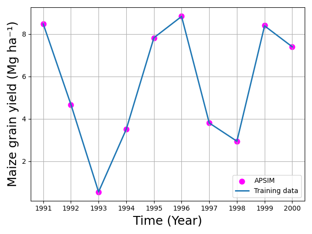
After the optimization is completed, compare the simulated results with the training dataset using the newly optimized parameters. The data attribute contains both the observed and simulated datasets, enabling direct comparison and evaluation of model performance.
import matplotlib.pyplot as plt
import os
# sns.relplot(x="year", y="y")
plt.figure(figsize=(8, 6))
df= de.data
df.eval('ayield =Yield/1000', inplace=True)
df.eval('oyield =observed/1000', inplace=True)
# observed → scatter points
plt.scatter(df["year"], df["ayield"], label="APSIM", s=60, color='red')
# predicted → line
plt.plot(df["year"], df["oyield"], label="Training data", linewidth=2)
plt.xlabel("Time (Year)", fontsize=18)
plt.ylabel("Maize grain yield (Mg ha⁻¹)", fontsize=18)
plt.title("") #Observed vs Predicted Yield Over Time
plt.legend()
plt.grid(True)
plt.tight_layout()
plt.savefig("figures.png")
os.startfile("figures.png")
plt.close()
Differential Evolution Performance and Comparison with Local Optimizers
In this example, Differential Evolution (DE) was used to calibrate two
APSIM parameters: [Phenology].GrainFilling.Target.FixedValue and
[Leaf].Photosynthesis.RUE.FixedValue. Although DE is robust for
non-convex and multi-modal landscapes, the results in this case show that
DE performed relatively poorly compared to simpler local optimization
methods, both in terms of computation time and final calibration
accuracy. These results were obtained using the default DE settings in
apsimNGpy. With additional parameter tuning—such as adjusting the
mutation factor (F), crossover rate (recombination), population size, or
evolution strategy—DE performance may improve and potentially match the
accuracy achieved by Nelder–Mead or Powell. However, such tuning increases
computational cost and may require multiple exploratory runs to identify
effective settings.
Full tutorial code:
from apsimNGpy.optimizer.minimize.single_mixed import MixedVariableOptimizer
from apsimNGpy.optimizer.problems.smp import MixedProblem
from apsimNGpy.optimizer.problems.variables import UniformVar, QrandintVar
from apsimNGpy.tests.unittests.test_factory import obs
if __name__ == "__main__":
    # -------------------------------------------------------------
    # 1. Define the mixed-variable optimization problem
    # -------------------------------------------------------------
    mp = MixedProblem(
        model="Maize",
        trainer_dataset=obs,
        pred_col="Yield",
        metric="wia",
        index="year",
        trainer_col="observed"
    )
    # A cultivar specific parameter
    cultivar_param = {
        "path": ".Simulations.Simulation.Field.Maize.CultivarFolder.Dekalb_XL82",
        "vtype": [QrandintVar(400, 900, q=10), UniformVar(0.8, 2.2)],  # Discrete step size of 2
        "start_value": [600, 1],
        "candidate_param": [
            '[Phenology].GrainFilling.Target.FixedValue',
            '[Leaf].Photosynthesis.RUE.FixedValue'],
        "other_params": {"sowed": True},
        "cultivar": True,  # Signals to apsimNGpy to treat it as a cultivar parameter
    }
    # Submit optimization factors
    mp.submit_factor(**cultivar_param)
    print(f" {mp.n_factors} optimization factors registered.")
    # -------------------------------------------------------------
    # 3. Configure and execute the optimizer
    # -------------------------------------------------------------
    minim = MixedVariableOptimizer(problem=mp)
    #_______________________________________________
    # use differential evolution
    de = minim.minimize_with_de(
        use_threads=True,
        updating="deferred",
        workers=14,  # Number of parallel workers
        popsize=30,  # Population size per generation
        constraints=(-1.1, -0.8),     # if metric indicator is one of wia, ccc , r2, slope the constraints must be negative
    )
    print("Differential evolution\n", de)
Local optimization examples
nelda = minim.minimize_with_local(method="Nelder-Mead")
print('nelda\n', nelda)
powell = minim.minimize_with_local(method="Powell")
print('Powell', powell)
lbfgs = minim.minimize_with_local(method="L-BFGS-B", options={
    "gtol": 1e-12,
    "ftol": 1e-12,
    "maxfun": 50000,
    "maxiter": 30000})
print(lbfgs)
bfgs = minim.minimize_with_local(method="BFGS")
print('bfgs\n', bfgs)

print("\nOptimization completed:")
# ----------------------------------
# now plot the results
# ---------------------------------
import matplotlib.pyplot as plt
import os
plt.figure(figsize=(8, 6))
df= de.data
df.eval('ayield =Yield/1000', inplace=True)
df.eval('oyield =observed/1000', inplace=True)
# observed → scatter points
plt.scatter(df["year"], df["ayield"], label="APSIM", s=60, color='red')
# predicted → line
plt.plot(df["year"], df["oyield"], label="Training data", linewidth=2)
plt.xlabel("Time (Year)", fontsize=18)
plt.ylabel("Maize grain yield (Mg ha⁻¹)", fontsize=18)
plt.title("") #Observed vs Predicted Yield Over Time
plt.legend()
plt.grid(True)
plt.tight_layout()
plt.savefig("figures.png")
if hasattr(os, 'startfile'):
   os.startfile("figures.png")
plt.close()